When solving many practical problems, it is not always necessary to characterize a random variable completely, that is, to determine the distribution laws. In addition, the construction of a function or a series of distributions for a discrete, and density - for a continuous random variable is cumbersome and unnecessary.

Sometimes it is enough to indicate individual numerical parameters that partially characterize the features of the distribution. It is necessary to know some average value of each random variable, around which its possible value is grouped, or the degree of dispersion of these values ​​relative to the average, etc.

The characteristics of the most significant features of the distribution are called numerical characteristics. random variable. With their help, it is easier to solve many probabilistic problems without defining distribution laws for them.

The most important characteristic of the position of a random variable on the number axis is expected value M[X]= a, which is sometimes called the mean of the random variable. For discrete random variable X with possible values x 1 , x 2 , … , x n and probabilities p 1 , p 2 ,… , p n it is determined by the formula

Considering that = 1, we can write

Thus, mathematical expectation a discrete random variable is the sum of the products of its possible values ​​by their probabilities. The arithmetic mean of the observed values ​​of a random variable with a large number of experiments approaches its mathematical expectation.

For continuous random variable X the mathematical expectation is determined not by the sum, but integral

where f(x) - distribution density of quantity X.

The mathematical expectation does not exist for all random variables. For some of them, the sum, or integral, diverges, and therefore there is no mathematical expectation. In these cases, for reasons of accuracy, the region of possible changes in the random variable should be limited X, for which the sum, or integral, will converge.

In practice, such characteristics of the position of a random variable as mode and median are also used.

Random variable modeits most probable value is called. In the general case, the mode and the mathematical expectation do not coincide.

The median of a random variableX is its value, relative to which it is equally probable to obtain a larger or smaller value of a random variable, that is, it is the abscissa of the point at which the area bounded by the distribution curve is divided in half. For a symmetric distribution, all three characteristics are the same.

In addition to the mathematical expectation, mode, and median, probability theory uses other characteristics, each of which describes a certain property of the distribution. For example, the numerical characteristics characterizing the dispersion of a random variable, that is, showing how closely its possible values ​​are grouped around the mathematical expectation, are the variance and the standard deviation. They significantly complement the random variable, since in practice random variables with equal mathematical expectations but different distributions are often encountered. When determining the scattering characteristics, use is made of the difference between a random variable X and its mathematical expectation, i.e.

where a = M[X] - expected value.

This difference is called centered random variable, corresponding value X, and denoted :

Variance of a random variable is the mathematical expectation of the square of the deviation of the value from its mathematical expectation, i.e.:

D [ X] = M [( X - a) 2], or

D [ X] = M [ 2 ].

The variance of a random variable is a convenient characteristic of the dispersion and dispersion of the values ​​of a random variable about its mathematical expectation. However, it is devoid of clarity, since it has the dimension of the square of a random variable.

For a visual characteristic of scattering, it is more convenient to use a quantity whose dimension coincides with the dimension of a random variable. This value is standard deviation a random variable that is the positive square root of its variance.

Mathematical expectation, mode, median, variance, standard deviation - the most commonly used numerical characteristics of random variables... When solving practical problems, when it is impossible to determine the distribution law, an approximate description of a random variable is its numerical characteristics, which express some property of distribution.

In addition to the main characteristics of the center distribution (mathematical expectation) and dispersion (variance), it is often necessary to describe other important characteristics of the distribution - symmetry and peakedness, which can be represented in terms of distribution moments.

The distribution of a random variable is completely specified if all its moments are known. However, many distributions can be fully described using the first four moments, which are not only parameters describing distributions, but are also important in the selection of empirical distributions, i.e., by calculating the numerical values ​​of the moments for a given statistical series and using special graphs, one can determine the distribution law.

In the theory of probability, moments of two types are distinguished: initial and central.

The initial moment of the kth order random variable T is the mathematical expectation of the quantity X k, i.e.

Therefore, for a discrete random variable, it is expressed by the sum

and for continuous - by the integral

Among the initial moments of a random variable, the moment of the first order, which is the mathematical expectation, is of particular importance. Higher-order initial moments are used mainly for calculating center moments.

The central moment of the kth order a random variable is called the mathematical expectation of a value ( X - M [X])k

where a = M [X].

For a discrete random variable, it is expressed by the sum

a for continuous - by the integral

Among the central moments of a random variable, of particular importance is central moment of the second order, which represents the variance of the random variable.

The central moment of the first order is always zero.

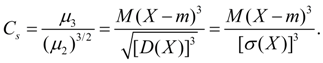
Third starting point characterizes the asymmetry (skewness) of the distribution and, according to the results of observations for discrete and continuous random variables, is determined by the corresponding expressions:

Since it has the dimension of a cube of a random variable, in order to obtain a dimensionless characteristic, m 3 divided by the standard deviation in the third power

The resulting value is called the coefficient of asymmetry and, depending on the sign, characterizes the positive ( As> 0) or negative ( As< 0) distribution skewness (Fig. 2.3).

71, Numerical characteristics of random variables are widely used in practice for calculating reliability indicators. In many questions of practice, there is no need to fully, exhaustively characterize a random variable. Often it is enough to indicate only the numerical parameters, to some extent characterizing the essential features of the distribution of the random variable, for example: mean , around which the possible values ​​of the random variable are grouped; number characterizing the scattering of a random variable relative to the mean value, etc. Numerical parameters that allow expressing in a concise form the most significant features of a random variable are called numerical characteristics of a random variable.

a) b)

Rice. 11 Determination of expected value

Numerical characteristics of random variables used in the theory of reliability are given in table. 1.

72, Expected value(mean value) of a continuous random variable, the possible values ​​of which belong to the interval , is a definite integral (Fig., 11, b)

. (26)

The mathematical expectation can be expressed in terms of the complement of the integral function. To do this, we substitute (11) into (26) and integrate by parts the resulting expression

, (27)

because and , then

. (28)

For non-negative random variables, the possible values ​​of which belong to the interval , formula (28) takes the form

. (29)

i.e. the mathematical expectation of a non-negative random variable, the possible values ​​of which belong to the interval , is numerically equal to the area under the graph of the addition of the integral function (Fig., 11, a).

73, Mean time to first failure according to statistical information is determined by the formula

, (30)

where is the operating time to the first failure i-th object; N- the number of tested objects.

The average resource, average service life, average recovery time, average shelf life are determined in the same way.

74, Scattering of a random variable around its mathematical expectation evaluated using variance of standard deviation(RMS) and coefficient of variation.

The variance of a continuous random variable X is the mathematical expectation of the square of the deviation of the random variable from its mathematical expectation and is calculated by the formula

. (31)

Dispersion has the dimension of the square of a random variable, which is not always convenient.

75, Standard deviation of the random variable is the square root of the variance and has the dimension of the random variable

. (32)

76, Coefficient of variation is a relative indicator of the dispersion of a random variable and is defined as the ratio of the standard deviation to the mathematical expectation

. (33)

77, Gamma - percentage value of a random variable- value of a random variable corresponding to a given probability the fact that the random variable will take a value greater than

. (34)

78, Gamma - the percentage value of a random variable can be determined by the integral function, its complement and differential function (Fig. 12). The gamma-percentage value of a random variable is a quantile of probability (Fig. 12, a)

. (35)

Reliability theory uses gamma percentage of resource, service life and shelf life(Table 1). Gamma percentage is called resource, service life, shelf life, which has (and exceeds) the percentage of objects of a given type.

a) b)

Fig. 12 Determination of the gamma-percentage value of a random variable

Gamma Percentage Resource characterizes durability at the selected level probability of non-destruction. The gamma-percentage resource is assigned taking into account the responsibility of the objects. For example, for rolling bearings, a 90 percent resource is most often used; for bearings of the most critical objects, a 95 percent resource and higher are chosen, bringing it closer to 100 percent, if the failure is dangerous for human life.

79, Median of random variable is its gamma percentage at ... For the median it is equally likely whether the random variable turns out to be T more or less than it, i.e.

Geometrically, the median is the abscissa of the intersection point of the cumulative distribution function and its complement (Fig. 12, b). The median can be interpreted as the abscissa of the point at which the ordinate of the differential function halves the area bounded by the distribution curve (Fig. 12, v).

The median of a random variable is used in the theory of reliability as a numerical characteristic of the resource, service life, shelf life (Table 1).

There is a functional relationship between the indicators of the reliability of objects. Knowledge of one of the functions
allows you to determine other indicators of reliability. A summary of the relationship between reliability indicators is given in table. 2.

Table 2. Functional relationship between reliability indicators

Expected value. Mathematical expectation discrete random variable NS that takes a finite number of values NSi with probabilities Ri, the sum is called:

Mathematical expectation continuous random variable NS is called the integral of the product of its values NS on the probability distribution f(x):

(6b)

Improper integral (6 b) is assumed to be absolutely convergent (otherwise it is said that the mathematical expectation M(NS) does not exist). The mathematical expectation characterizes mean random variable NS... Its dimension coincides with the dimension of a random variable.

Mathematical expectation properties:

Dispersion. Dispersion random variable NS the number is called:

The variance is scattering characteristic values ​​of a random variable NS relative to its mean M(NS). The dimension of the variance is equal to the dimension of the random variable squared. Based on the definitions of variance (8) and mathematical expectation (5) for a discrete random variable and (6) for a continuous random variable, we obtain similar expressions for the variance:

(9)

Here m = M(NS).

Dispersion properties:

Mean square deviation:

(11)

Since the dimension of the standard deviation is the same as that of a random variable, it is more often than the variance used as a measure of scattering.

Distribution moments. The concepts of mathematical expectation and variance are special cases of a more general concept for the numerical characteristics of random variables - distribution moments... The moments of distribution of a random variable are introduced as the mathematical expectations of some of the simplest functions of a random variable. So, a moment of order k relative to point NS 0 is called the mathematical expectation M(NS–NS 0 )k... Moments relative to the origin NS= 0 are called starting points and are designated:

(12)

The initial moment of the first order is the center of the distribution of the considered random variable:

(13)

Moments relative to the distribution center NS= m are called focal points and are designated:

(14)

It follows from (7) that the central moment of the first order is always zero:

The central moments do not depend on the origin of the values ​​of the random variable, since when shifted by a constant value WITH its distribution center is shifted by the same value WITH, and the deviation from the center does not change: NS – m = (NS – WITH) – (m – WITH).
It is now obvious that dispersion- this is central moment of the second order:

Asymmetry. Central moment of the third order:

(17)

serves to assess distribution asymmetry... If the distribution is symmetric about the point NS= m, then the central moment of the third order will be equal to zero (like all central moments of odd orders). Therefore, if the central moment of the third order is nonzero, then the distribution cannot be symmetric. The magnitude of the asymmetry is estimated using the dimensionless asymmetry coefficient:

(18)

The sign of the asymmetry coefficient (18) indicates right-sided or left-sided asymmetry (Fig. 2).

Rice. 2. Types of distribution asymmetry.

Excess. The central moment of the fourth order:

(19)

serves to assess the so-called excess, which determines the degree of steepness (peakedness) of the distribution curve near the distribution center with respect to the normal distribution curve. Since for a normal distribution, then the value is taken as kurtosis:

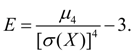(20)

In fig. 3 shows examples of distribution curves with different kurtosis values. For normal distribution E= 0. Curves that are more peaked than normal have a positive kurtosis, more flat-topped ones have negative kurtosis.

Rice. 3. Curves of distribution with different degrees of steepness (kurtosis).

Higher-order moments are usually not used in engineering applications of mathematical statistics.

Fashion discrete a random variable is its most probable value. Fashion continuous random variable is called its value at which the probability density is maximum (Fig. 2). If the distribution curve has one maximum, then the distribution is called unimodal... If the distribution curve has more than one maximum, then the distribution is called polymodal... Sometimes there are distributions whose curves have not a maximum, but a minimum. Such distributions are called anti-modal... In the general case, the mode and the mathematical expectation of a random variable do not coincide. In a particular case, for modal, i.e. having a mode, symmetric distribution and provided that there is a mathematical expectation, the latter coincides with the mode and the center of symmetry of the distribution.

Median random variable NS Is its meaning Me, for which the equality holds: i.e. it is equally probable that the random variable NS will be less or more Me... Geometrically median Is the abscissa of the point at which the area under the distribution curve is halved (Fig. 2). In the case of a symmetric modal distribution, the median, mode, and mathematical expectation are the same.

RANDOM VALUES AND LAWS OF THEIR DISTRIBUTION.

Random is called such a value that takes on values ​​depending on the coincidence of random circumstances. Distinguish discrete and random continuous magnitudes.

Discrete a quantity is called if it takes a countable set of values. ( Example: the number of patients at the doctor's appointment, the number of letters on the page, the number of molecules in a given volume).

Continuous is a quantity that can take values ​​within a certain interval. ( Example: air temperature, body weight, human height, etc.)

Distribution law A random variable is a set of possible values ​​of this quantity and, corresponding to these values, probabilities (or frequencies of occurrence).

PRI me R:

Numerical characteristics of random variables.

In many cases, along with the distribution of a random variable or instead of it, information about these quantities can be given by numerical parameters, called numerical characteristics of a random variable ... The most common ones:

1 .Expected value - (mean value) of a random variable is the sum of the products of all its possible values ​​by the probabilities of these values:

2 .Dispersion random variable:

3 .Root mean square deviation :

Rule "THREE SIGMA" - if a random variable is distributed according to the normal law, then the deviation of this value from the mean value in absolute value does not exceed three times the standard deviation

Gaussian law - normal distribution law

Often there are quantities distributed over normal law (Gauss's law). main feature : it is a limiting law, which is approached by other distribution laws.

A random variable is distributed according to the normal law if its probability density looks like:

M (X) - mathematical expectation of a random variable;

 - standard deviation.

Probability density (distribution function) shows how the probability changes relative to the interval dx a random variable, depending on the value of the quantity itself:

Basic concepts of mathematical statistics

Math statistics - a branch of applied mathematics, directly adjacent to the theory of probability. The main difference between mathematical statistics and probability theory is that in mathematical statistics, it is not actions on the distribution laws and numerical characteristics of random variables that are considered, but approximate methods for finding these laws and numerical characteristics based on the results of experiments.

Basic concepts mathematical statistics are:

General population;

sample;

variation range;

fashion;

median;

percentile,

frequency polygon,

bar graph.

General population - a large statistical population, from which some of the objects are selected for research

(Example: the entire population of the region, students of universities of a given city, etc.)

Sample (sample population) - a set of objects selected from the general population.

Variational series - statistical distribution, consisting of a variant (values ​​of a random variable) and the corresponding frequencies.

Example:

x - value of a random variable (mass of girls aged 10 years);

m - frequency of occurrence.

Fashion - the value of a random variable, which corresponds to the highest frequency of occurrence. (In the above example, the mod corresponds to the value of 24 kg, it is found more often than others: m = 20).

Median - the value of a random variable that divides the distribution in half: half of the values ​​are located to the right of the median, half (no more) - to the left.

Example:

1, 1, 1, 1, 1. 1, 2, 2, 2, 3 , 3, 4, 4, 5, 5, 5, 5, 6, 6, 7 , 7, 7, 7, 7, 7, 8, 8, 8, 8, 8 , 8, 9, 9, 9, 10, 10, 10, 10, 10, 10

In the example, we observe 40 values ​​of a random variable. All values ​​are arranged in ascending order based on their frequency of occurrence. You can see that 20 (half) of 40 values ​​are located to the right of the highlighted value 7. Therefore, 7 is the median.

To characterize the scatter, we find the values ​​that did not exceed 25 and 75% of the measurement results. These values ​​are called 25th and 75th percentiles ... If the median halves the distribution, then the 25th and 75th percentiles are cut off by a quarter. (The median itself, by the way, can be considered the 50th percentile.) As you can see from the example, the 25th and 75th percentiles are 3 and 8, respectively.

Use discrete (point) statistical distribution and continuous (interval) statistical distribution.

For clarity, statistical distributions are depicted graphically in the form frequency polygon or - histograms .

Frequency polygon - polyline, segments of which connect points with coordinates ( x 1 , m 1 ), (x 2 , m 2 ), ..., or for polygon of relative frequencies - with coordinates ( x 1 ,R * 1 ), (x 2 ,R * 2 ), ... (Fig. 1).

mm i / nf (x)

x x

Fig. 1 Fig. 2

Frequency histogram - a set of adjacent rectangles built on one straight line (Fig. 2), the bases of the rectangles are the same and equal dx , and the heights are equal to the ratio of the frequency to dx , or R * To dx (probability density).

Example: