PROPERTIES OF FUNCTIONS CONTINUOUS ON AN INTERVIEW

Let's consider some properties of functions continuous on an interval. We present these properties without proof.

Function y = f(x) called continuous on the segment [a, b], if it is continuous at all internal points of this segment, and at its ends, i.e. at points a And b, is continuous on the right and left, respectively.

Theorem 1. A function continuous on the interval [ a, b], at least at one point of this segment takes the greatest value and at least at one point the smallest.

The theorem states that if a function y = f(x) is continuous on the interval [ a, b], then there is at least one point x 1 Î [ a, b] such that the value of the function f(x) at this point will be the largest of all its values ​​on this segment: f(x 1) ≥ f(x). Similarly, there is such a point x 2, in which the function value will be the smallest of all values ​​on the segment: f(x 1) ≤ f(x).

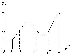
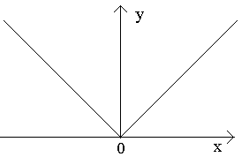
It is clear that there may be several such points; for example, the figure shows that the function f(x) takes the smallest value at two points x 2 And x 2 ".

Comment. The statement of the theorem can become incorrect if we consider the value of the function on the interval ( a, b). Indeed, if we consider the function y = x on (0, 2), then it is continuous on this interval, but does not reach either the largest or the smallest values ​​in it: it reaches these values ​​at the ends of the interval, but the ends do not belong to our domain.

Also, the theorem ceases to be true for discontinuous functions. Give an example.

Consequence. If the function f(x) is continuous on [ a, b], then it is limited on this segment.

Theorem 2. Let the function y = f(x) is continuous on the interval [ a, b] and at the ends of this segment takes values ​​of different signs, then there is at least one point inside the segment x = C, in which the function goes to zero: f(C)= 0, where a< C< b

This theorem has a simple geometric meaning: if the points of the graph of a continuous function y = f(x), corresponding to the ends of the segment [ a, b] lie on opposite sides of the axis Ox, then this graph intersects the axis at at least one point of the segment Ox. Discontinuous functions may not have this property.

This theorem admits the following generalization.

Theorem 3 (intermediate value theorem). Let the function y = f(x) is continuous on the interval [ a, b] And f(a) = A, f(b) = B. Then for any number C, concluded between A And B, there is such a point inside this segment CÎ [ a, b], What f(c) = C.

This theorem is geometrically obvious. Consider the graph of the function y = f(x). Let f(a) = A, f(b) = B. Then any straight line y = C, Where C– any number between A And B, will intersect the graph of the function at least at one point. The abscissa of the intersection point will be that value x = C, at which f(c) = C.

Thus, a continuous function, moving from one value to another, necessarily passes through all intermediate values. In particular:

Consequence. If the function y = f(x) is continuous over a certain interval and takes the largest and smallest values, then on this interval it takes at least once any value contained between its smallest and largest values.

DERIVATIVE AND ITS APPLICATIONS. DEFINITION OF DERIVATIVE

Let us have some function y=f(x), defined on some interval. For each argument value x from this interval the function y=f(x) has a certain meaning.

Consider two argument values: initial x 0 and new x.

Difference x–x 0 is called by incrementing the argument x at the point x 0 and is denoted Δx. Thus, Δx = x – x 0 (the argument increment can be either positive or negative). From this equality it follows that x=x 0 +Δx, i.e. the initial value of the variable has received some increment. Then, if at the point x 0 function value was f(x 0 ), then at a new point x the function will take the value f(x) = f(x 0 +Δx).

Difference y–y 0 = f(x) – f(x 0 ) called function increment y = f(x) at the point x 0 and is indicated by the symbol Δy. Thus,

Typically the initial value of the argument x 0 is considered fixed, and the new value x– variable. Then y 0 = f(x 0 ) turns out to be constant, and y = f(x)– variable. Increments Δy And Δx will also be variables and formula (1) shows that Dy is a function of a variable Δx.

Let's create the ratio of the increment of the function to the increment of the argument

Let us find the limit of this ratio at Δx→0. If this limit exists, then it is called the derivative of this function f(x) at the point x 0 and denote f "(x 0). So,

Derivative this function y = f(x) at the point x 0 is called the limit of the function increment ratio Δ y to the argument increment Δ x, when the latter arbitrarily tends to zero.

Note that for the same function the derivative at different points x can take on different values, i.e. the derivative can be considered as a function of the argument x. This function is designated f "(x)

The derivative is denoted by the symbols f "(x),y", . The specific value of the derivative at x = a denoted by f "(a) or y "| x=a.

The operation of finding the derivative of a function f(x) is called differentiation of this function.

To directly find the derivative by definition, you can use the following: rule of thumb:

Examples.

MECHANICAL SENSE OF DERIVATIVE

It is known from physics that the law of uniform motion has the form s = v t, Where s– the path traveled to the moment of time t, v– speed of uniform motion.

However, because Most movements occurring in nature are uneven, then in general the speed, and, consequently, the distance s will depend on time t, i.e. will be a function of time.

So, let a material point move in a straight line in one direction according to the law s=s(t).

Let's mark a certain point in time t 0 . At this point the point has passed the path s=s(t 0 ). Let's determine the speed v material point at a moment in time t 0 .

To do this, let's consider some other point in time t 0 + Δ t. It corresponds to the traveled path s =s(t 0 + Δ t). Then over a period of time Δ t the point has traveled the path Δs =s(t 0 + Δ t)–s(t).

Let's consider the attitude. It is called the average speed in the time interval Δ t. The average speed cannot accurately characterize the speed of movement of a point at the moment t 0 (because the movement is uneven). In order to more accurately express this true speed using the average speed, you need to take a shorter period of time Δ t.

So, the speed of movement at a given moment in time t 0 (instantaneous speed) is the limit of average speed in the interval from t 0 to t 0 +Δ t, when Δ t→0:

,

those. uneven speed this is the derivative of the distance traveled with respect to time.

GEOMETRICAL MEANING OF DERIVATIVE

Let us first introduce the definition of a tangent to a curve at a given point.

Let us have a curve and a fixed point on it M 0(see figure). Consider another point M this curve and draw a secant M 0 M. If the point M begins to move along the curve, and the point M 0 remains motionless, then the secant changes its position. If, with unlimited approximation of the point M along a curve to a point M 0 on any side the secant tends to occupy the position of a certain straight line M 0 T, then straight M 0 T called the tangent to the curve at a given point M 0.

That., tangent to the curve at a given point M 0 called the limit position of the secant M 0 M when point M tends along the curve to a point M 0.

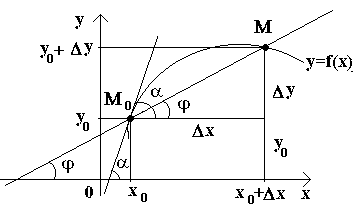
Let us now consider the continuous function y=f(x) and the curve corresponding to this function. At some value X 0 function takes value y 0 =f(x 0). These values x 0 and y 0 on the curve corresponds to a point M 0 (x 0 ; y 0). Let's give the argument x 0 increment Δ X. The new value of the argument corresponds to the incremented value of the function y 0 +Δ y=f(x 0 –Δ x). We get the point M(x 0+Δ x; y 0+Δ y). Let's draw a secant M 0 M and denote by φ the angle formed by a secant with the positive direction of the axis Ox. Let's create a relation and note that .

If now Δ x→0, then due to the continuity of the function Δ at→0, and therefore the point M, moving along a curve, approaches the point without limit M 0. Then the secant M 0 M will tend to take the position of a tangent to the curve at the point M 0, and the angle φ→α at Δ x→0, where α denotes the angle between the tangent and the positive direction of the axis Ox. Since the function tan φ continuously depends on φ for φ≠π/2, then for φ→α tan φ → tan α and, therefore, the slope of the tangent will be:

those. f "(x)= tg α .

Thus, geometrically y "(x 0) represents the slope of the tangent to the graph of this function at the point x 0, i.e. for a given argument value x, the derivative is equal to the tangent of the angle formed by the tangent to the graph of the function f(x) at the appropriate point M 0 (x; y) with positive axis direction Ox.

Example. Find the slope of the tangent to the curve y = x 2 at point M(-1; 1).

We have already seen earlier that ( x 2)" = 2X. But the angular coefficient of the tangent to the curve is tan α = y"| x=-1 = – 2.

DIFFERENTIABILITY OF FUNCTIONS. CONTINUITY OF DIFFERENTIABLE FUNCTION

Function y=f(x) called differentiable at some point x 0 if it has a certain derivative at this point, i.e. if the limit of the relationship exists and is finite.

If a function is differentiable at each point of a certain segment [ A; b] or interval ( A; b), then they say that she differentiable on the segment [ A; b] or, respectively, in the interval ( A; b).

The following theorem is valid, establishing the connection between differentiable and continuous functions.

Theorem. If the function y=f(x) differentiable at some point x 0, then it is continuous at this point.

Thus, from the differentiability of a function, its continuity follows.

Proof. If , That

,

where α is an infinitesimal quantity, i.e. a quantity tending to zero as Δ x→0. But then

Δ y=f "(x 0) Δ x+αΔ x=> Δ y→0 at Δ x→0, i.e. f(x) – f(x 0)→0 at x→x 0 , which means that the function f(x) continuous at a point x 0 . Q.E.D.

Thus, the function cannot have a derivative at discontinuity points. The converse is not true: there are continuous functions that are not differentiable at some points (that is, do not have a derivative at these points).

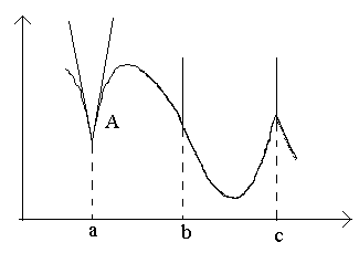
Consider the points in the figure a, b, c.

At the point a at Δ x→0 the ratio has no limit (since the one-sided limits are different for Δ x→0–0 and Δ x→0+0). At the point A graph there is no defined tangent, but there are two different one-way tangents with slopes To 1 and To 2. This type of point is called corner point.

At the point b at Δ x The →0 ratio is a constant sign infinitely large quantity. The function has infinite derivative. At this point the graph has a vertical tangent. Point type – “inflection point” of a vertical tangent.

At the point c one-sided derivatives are infinitely large quantities of different signs. At this point the graph has two merged vertical tangents. Type – “return point” with a vertical tangent – ​​a special case of a corner point.

The figures below show where the function can reach its smallest and largest value. In the left figure, the smallest and largest values ​​are fixed at the points of local minimum and maximum of the function. In the right picture - at the ends of the segment.

If the function y = f(x) is continuous on the interval [ a, b] , then it reaches on this segment least And highest values . This, as already mentioned, can happen either in extremum points, or at the ends of the segment. Therefore, to find least And the largest values ​​of the function , continuous on the interval [ a, b] , you need to calculate its values ​​in all critical points and at the ends of the segment, and then choose the smallest and largest from them.

Let, for example, you want to determine the largest value of the function f(x) on the segment [ a, b] . To do this, you need to find all its critical points lying on [ a, b] .

Critical point called the point at which function defined, and her derivative either equal to zero or does not exist. Then you should calculate the values ​​of the function at the critical points. And finally, one should compare the values ​​of the function at critical points and at the ends of the segment ( f(a) And f(b)). The largest of these numbers will be the largest value of the function on the segment [a, b] .

Problems of finding smallest function values .

We look for the smallest and largest values ​​of the function together

Example 1. Find the smallest and largest values ​​of a function on the segment [-1, 2] .

Solution. Find the derivative of this function. Let's equate the derivative to zero () and get two critical points: and . To find the smallest and largest values ​​of a function on a given segment, it is enough to calculate its values ​​at the ends of the segment and at the point, since the point does not belong to the segment [-1, 2]. These function values ​​are: , , . It follows that smallest function value(indicated in red on the graph below), equal to -7, is achieved at the right end of the segment - at point , and greatest(also red on the graph), equals 9, - at the critical point.

If a function is continuous in a certain interval and this interval is not a segment (but is, for example, an interval; the difference between an interval and a segment: the boundary points of the interval are not included in the interval, but the boundary points of the segment are included in the segment), then among the values ​​of the function there may not be to be the smallest and the greatest. So, for example, the function shown in the figure below is continuous on ]-∞, +∞[ and does not have the greatest value.

However, for any interval (closed, open or infinite), the following property of continuous functions is true.

For self-checking during calculations, you can use online derivative calculator .

Example 4. Find the smallest and largest values ​​of a function on the segment [-1, 3] .

Solution. We find the derivative of this function as the derivative of the quotient:

.

We equate the derivative to zero, which gives us one critical point: . It belongs to the segment [-1, 3] . To find the smallest and largest values ​​of a function on a given segment, we find its values ​​at the ends of the segment and at the found critical point:

Let's compare these values. Conclusion: equal to -5/13, at point and highest value equal to 1 at point .

We continue to look for the smallest and largest values ​​of the function together

There are teachers who, on the topic of finding the smallest and largest values ​​of a function, do not give students examples to solve that are more complex than those just discussed, that is, those in which the function is a polynomial or a fraction, the numerator and denominator of which are polynomials. But we will not limit ourselves to such examples, since among teachers there are those who like to force students to think in full (the table of derivatives). Therefore, the logarithm and trigonometric function will be used.

Example 8. Find the smallest and largest values ​​of a function on the segment .

Solution. We find the derivative of this function as derivative of the product :

We equate the derivative to zero, which gives one critical point: . It belongs to the segment. To find the smallest and largest values ​​of a function on a given segment, we find its values ​​at the ends of the segment and at the found critical point:

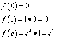
Result of all actions: the function reaches its minimum value, equal to 0, at the point and at the point and highest value, equal e², at the point.

For self-checking during calculations, you can use online derivative calculator .

Example 9. Find the smallest and largest values ​​of a function on the segment .

Solution. Find the derivative of this function:

We equate the derivative to zero:

The only critical point belongs to the segment. To find the smallest and largest values ​​of a function on a given segment, we find its values ​​at the ends of the segment and at the found critical point:

Conclusion: the function reaches its minimum value, equal to , at the point and highest value, equal , at the point .

In applied extremal problems, finding the smallest (maximum) values ​​of a function, as a rule, comes down to finding the minimum (maximum). But it is not the minimums or maximums themselves that are of greater practical interest, but those values ​​of the argument at which they are achieved. When solving applied problems, an additional difficulty arises - composing functions that describe the phenomenon or process under consideration.

Example 10. A tank with a capacity of 4, having the shape of a parallelepiped with a square base and open at the top, must be tinned. What size should the tank be so that the least amount of material is used to cover it?

Solution. Let x- base side, h- tank height, S- its surface area without cover, V- its volume. The surface area of ​​the tank is expressed by the formula, i.e. is a function of two variables. To express S as a function of one variable, we use the fact that , from where . Substituting the found expression h into the formula for S:

Let's examine this function to its extremum. It is defined and differentiable everywhere in ]0, +∞[ , and

.

We equate the derivative to zero () and find the critical point. In addition, when the derivative does not exist, but this value is not included in the domain of definition and therefore cannot be an extremum point. So, this is the only critical point. Let's check it for the presence of an extremum using the second sufficient sign. Let's find the second derivative. When the second derivative is greater than zero (). This means that when the function reaches a minimum . Since this minimum is the only extremum of this function, it is its smallest value. So, the side of the base of the tank should be 2 m, and its height should be .

For self-checking during calculations, you can use

From a practical point of view, the greatest interest is in using the derivative to find the largest and smallest values ​​of a function. What is this connected with? Maximizing profits, minimizing costs, determining the optimal load of equipment... In other words, in many areas of life we ​​have to solve problems of optimizing some parameters. And these are the tasks of finding the largest and smallest values ​​of a function.

It should be noted that the largest and smallest values ​​of a function are usually sought on a certain interval X, which is either the entire domain of the function or part of the domain of definition. The interval X itself can be a segment, an open interval , an infinite interval.

In this article we will talk about finding the largest and smallest values ​​of an explicitly defined function of one variable y=f(x) .

Page navigation.

The largest and smallest value of a function - definitions, illustrations.

Let's briefly look at the main definitions.

The largest value of the function that for anyone inequality is true.

The smallest value of the function y=f(x) on the interval X is called such a value that for anyone inequality is true.

These definitions are intuitive: the largest (smallest) value of a function is the largest (smallest) accepted value on the interval under consideration at the abscissa.

Stationary points– these are the values ​​of the argument at which the derivative of the function becomes zero.

Why do we need stationary points when finding the largest and smallest values? The answer to this question is given by Fermat's theorem. From this theorem it follows that if a differentiable function has an extremum (local minimum or local maximum) at some point, then this point is stationary. Thus, the function often takes its largest (smallest) value on the interval X at one of the stationary points from this interval.

Also, a function can often take on its largest and smallest values ​​at points at which the first derivative of this function does not exist, and the function itself is defined.

Let’s immediately answer one of the most common questions on this topic: “Is it always possible to determine the largest (smallest) value of a function”? No not always. Sometimes the boundaries of the interval X coincide with the boundaries of the domain of definition of the function, or the interval X is infinite. And some functions at infinity and at the boundaries of the domain of definition can take on both infinitely large and infinitely small values. In these cases, nothing can be said about the largest and smallest value of the function.

For clarity, we will give a graphic illustration. Look at the pictures and a lot will become clearer.

On the segment

In the first figure, the function takes the largest (max y) and smallest (min y) values ​​at stationary points located inside the segment [-6;6].

Consider the case depicted in the second figure. Let's change the segment to . In this example, the smallest value of the function is achieved at a stationary point, and the largest at the point with the abscissa corresponding to the right boundary of the interval.

In Figure 3, the boundary points of the segment [-3;2] are the abscissas of the points corresponding to the largest and smallest value of the function.

On an open interval

In the fourth figure, the function takes the largest (max y) and smallest (min y) values ​​at stationary points located inside the open interval (-6;6).

On the interval , no conclusions can be drawn about the largest value.

At infinity

In the example presented in the seventh figure, the function takes the largest value (max y) at a stationary point with abscissa x=1, and the smallest value (min y) is achieved on the right boundary of the interval. At minus infinity, the function values ​​asymptotically approach y=3.

Over the interval, the function reaches neither the smallest nor the largest value. As x=2 approaches from the right, the function values ​​tend to minus infinity (the line x=2 is a vertical asymptote), and as the abscissa tends to plus infinity, the function values ​​asymptotically approach y=3. A graphic illustration of this example is shown in Figure 8.

Algorithm for finding the largest and smallest values ​​of a continuous function on a segment.

Let us write an algorithm that allows us to find the largest and smallest values ​​of a function on a segment.

1. We find the domain of definition of the function and check whether it contains the entire segment.
2. We find all the points at which the first derivative does not exist and which are contained in the segment (usually such points are found in functions with an argument under the modulus sign and in power functions with a fractional-rational exponent). If there are no such points, then move on to the next point.
3. We determine all stationary points falling within the segment. To do this, we equate it to zero, solve the resulting equation and select suitable roots. If there are no stationary points or none of them fall into the segment, then move on to the next point.
4. We calculate the values ​​of the function at selected stationary points (if any), at points at which the first derivative does not exist (if any), as well as at x=a and x=b.
5. From the obtained values ​​of the function, we select the largest and smallest - they will be the required largest and smallest values ​​of the function, respectively.

Let's analyze the algorithm for solving an example to find the largest and smallest values ​​of a function on a segment.

Example.

Find the largest and smallest value of a function

• on the segment ;
• on the segment [-4;-1] .

Solution.

The domain of definition of a function is the entire set of real numbers, with the exception of zero, that is. Both segments fall within the definition domain.

Find the derivative of the function with respect to:

Obviously, the derivative of the function exists at all points of the segments and [-4;-1].

We determine stationary points from the equation. The only real root is x=2. This stationary point falls into the first segment.

For the first case, we calculate the values ​​of the function at the ends of the segment and at the stationary point, that is, for x=1, x=2 and x=4:

Therefore, the greatest value of the function is achieved at x=1, and the smallest value – at x=2.

For the second case, we calculate the function values ​​only at the ends of the segment [-4;-1] (since it does not contain a single stationary point):

Solution.

Let's start with the domain of the function. The square trinomial in the denominator of the fraction must not vanish:

It is easy to check that all intervals from the problem statement belong to the domain of definition of the function.

Let's differentiate the function:

Obviously, the derivative exists throughout the entire domain of definition of the function.

Let's find stationary points. The derivative goes to zero at . This stationary point falls within the intervals (-3;1] and (-3;2).

Now you can compare the results obtained at each point with the graph of the function. Blue dotted lines indicate asymptotes.

At this point we can finish with finding the largest and smallest values ​​of the function. The algorithms discussed in this article allow you to get results with a minimum of actions. However, it can be useful to first determine the intervals of increase and decrease of the function and only after that draw conclusions about the largest and smallest values ​​of the function on any interval. This gives a clearer picture and rigorous justification for the results.

Definition3 . 3 Let be some function, its domain of definition, and some (open) interval (maybe with and/or ) 7 . Let's call the function continuous on the interval, if continuous at any point, that is, for any there is (in abbreviated form:

Let now be a (closed) segment in . Let's call the function continuous on the segment, if continuous on the interval, continuous on the right at the point and continuous on the left at the point, that is

Example3 . 13 Consider the function (Heaviside function) on the segment , . Then it is continuous on the segment (despite the fact that at the point it has a discontinuity of the first kind).

Fig. 3.15. Graph of the Heaviside function

A similar definition can be given for half-intervals of the form and , including cases and . However, we can generalize this definition to the case of an arbitrary subset as follows. Let us first introduce the concept induced to bases: let be a base all of whose endings have non-empty intersections with . Let us denote by and consider the set of all . It is then easy to check that the set will be the base. Thus, for the bases , and , where , and are the bases of unpunctured two-sided (left, right, respectively) neighborhoods of a point (see their definition at the beginning of the current chapter).

Definition3 . 4 Let's call the function continuous on the set, If

It is easy to see that then at and at this definition coincides with those given above specifically for the interval and segment.

Recall that all elementary functions are continuous at all points of their domains of definition and, therefore, continuous on any intervals and segments lying in their domains of definition.

Since continuity on an interval and segment is defined pointwise, the theorem holds, which is an immediate consequence of Theorem 3.1:

Theorem3 . 5 Let And -- functions and -- interval or segment lying in . Let And continuous for . Then the functions , , continuous for . If in addition in front of everyone , then the function is also continuous on .

The following statement follows from this theorem, just as from Theorem 3.1 - Proposition 3.3:

Offer3 . 4 A bunch of all functions continuous on an interval or segment -- this is a linear space:

A more complex property of a continuous function is expressed by the following theorem.

Theorem3 . 6 (about the root of a continuous function) Let the function continuous on the segment , and And -- numbers of different signs. (For definiteness, we will assume that , A .) Then there is at least one such value , What (that is, there is at least one root equations ).

Proof. Let's look at the middle of the segment. Then it's either, or, or. In the first case, the root is found: this is . In the remaining two cases, consider that part of the segment at the ends of which the function takes values ​​of different signs: in case or in case . We denote the selected half of the segment by and apply the same procedure to it: divide it into two halves and , where , and find . In case the root is found; in the case we further consider the segment , in case - segment etc.

Fig. 3.16. Consecutive divisions of a segment in half

We get that either at some step the root will be found, or a system of nested segments will be constructed

in which each subsequent segment is half as long as the previous one. The sequence is non-decreasing and bounded from above (for example, by the number); therefore (by Theorem 2.13), it has a limit. Subsequence - non-increasing and bounded below (for example, by the number ); this means there is a limit. Since the lengths of the segments form a decreasing geometric progression (with denominator ), they tend to 0, and , that is . Let's put it now. Then

And

since the function is continuous. However, by the construction of the sequences and , and , so that, by the theorem on passing to the limit in the inequality (Theorem 2.7), and , that is, and . This means that , and is the root of the equation.

Example3 . 14 Consider the function on the segment. Since and are numbers of different signs, the function turns to 0 at some point in the interval. This means that the equation has a root.

Fig. 3.17. Graphical representation of the root of the equation

The proven theorem actually gives us a way to find the root, at least approximate, with any degree of accuracy specified in advance. This is the method of dividing a segment in half, described in the proof of the theorem. We will get acquainted with this and other, more effective, methods of approximately finding the root in more detail below, after we study the concept and properties of a derivative.

Note that the theorem does not state that if its conditions are met, then the root is unique. As the following figure shows, there can be more than one root (there are 3 in the figure).

Fig. 3.18. Several roots of a function that takes values ​​of different signs at the ends of the segment

However, if a function monotonically increases or monotonically decreases on a segment, at the ends of which it takes values ​​of different signs, then the root is unique, since a strictly monotone function takes each of its values ​​at exactly one point, including the value 0.

Fig. 3.19. A monotonic function cannot have more than one root

An immediate consequence of the theorem on the root of a continuous function is the following theorem, which in itself is very important in mathematical analysis.

Theorem3 . 7 (about the intermediate value of a continuous function) Let the function continuous on the segment And (for definiteness we will assume that ). Let -- some number lying between And . Then there is such a point , What .

Fig. 3.20. Continuous function takes any intermediate value

Proof. Consider the helper function , Where . Then And . The function is obviously continuous, and by the previous theorem there is a point such that . But this equality means that .

Note that if the function is not continuous, then it may not take all intermediate values. For example, the Heaviside function (see Example 3.13) takes the values ​​, , but nowhere, including on the interval, does it take, say, an intermediate value. The fact is that the Heaviside function has a discontinuity at a point lying exactly in the interval.

To further study the properties of functions continuous on an interval, we will need the following subtle property of the system of real numbers (we already mentioned it in Chapter 2 in connection with the theorem on the limit of a monotonically increasing bounded function): for any set bounded below (that is, such that for all and some; the number is called bottom edge sets) available exact bottom edge, that is, the largest of the numbers such that for all . Similarly, if a set is bounded above, then it has exact upper bound: this is the smallest of top faces(for which for all).

Fig. 3.21. Lower and upper bounds of a bounded set

If , then there is a non-increasing sequence of points that tends to . In the same way, if , then there is a non-decreasing sequence of points that tends to .

If a point belongs to the set, then it is the smallest element of this set: ; similarly if , That .

In addition, for further we will need the following

Lemma3 . 1 Let -- continuous function on a segment , and many those points , in which (or , or ) is not empty. Then in abundance there is a smallest value , such that in front of everyone .

Fig. 3.22. The smallest argument at which the function takes the specified value

Proof. Since it is a bounded set (it is part of a segment), it has an infimum. Then there exists a non-increasing sequence , , such that for . Moreover, by the definition of a set. Therefore, passing to the limit, we obtain, on the one hand,

and on the other hand, due to the continuity of the function,

This means , so the point belongs to the set and .

In the case when the set is defined by the inequality , we have for all and by the theorem on passing to the limit in the inequality we obtain

from where , which means that and . Similarly, in the case of inequality, passing to the limit in the inequality gives

from where, and.

Theorem3 . 8 (about the boundedness of a continuous function) Let the function continuous on the segment . Then limited to , that is, there is such a constant , What in front of everyone .

Fig. 3.23. A function continuous on a segment is bounded

Proof. Let us assume the opposite: let it not be limited, for example, from above. Then all sets , , , are not empty. By the previous lemma, each of these sets has the smallest value , . Let's show that

Really, . If any point from , for example, lies between and , then

that is, an intermediate value between and . This means, by the theorem about the intermediate value of a continuous function, there exists a point such that , And . But, contrary to the assumption that - the smallest value of the set. It follows that for all .

In the same way, it is further proven that for all , for all , etc. So, is an increasing sequence bounded above by the number . Therefore it exists. From the continuity of the function it follows that there is , But at , so there is no limit. The resulting contradiction proves that the function is bounded above.

It is proved in a similar way that it is bounded from below, which implies the statement of the theorem.

Obviously, it is impossible to weaken the conditions of the theorem: if a function is not continuous, then it does not have to be bounded on an interval (we give as an example the function

on the segment. This function is not bounded on the interval, since at has a discontinuity point of the second kind, such that at . It is also impossible to replace a segment in the condition of the theorem with an interval or half-interval: as an example, consider the same function on a half-interval. The function is continuous on this half-interval, but unbounded, due to the fact that at .

Finding the best constants that can be used to limit a function from above and below on a given interval naturally leads us to the problem of finding the minimum and maximum of a continuous function on this interval. The possibility of solving this problem is described by the following theorem.

Theorem3 . 9 (about reaching an extremum by a continuous function) Let the function continuous on the segment . Then there is a point , such that in front of everyone (that is -- minimum point: ), and there is a point , such that in front of everyone (that is -- maximum point: ). In other words, the minimum and maximum 8 values ​​of a continuous function on a segment exist and are achieved at some points And this segment.

Fig. 3.24. A function continuous on a segment reaches a maximum and a minimum

Proof. Since, according to the previous theorem, the function is bounded by above, then there is an exact upper bound for the values ​​of the function by -- number . Thus, the sets , ,..., ,..., are not empty, and by the previous lemma they contain the smallest values ​​: , . These do not decrease (this statement is proven in exactly the same way as in the previous theorem):

and are limited from above by . Therefore, according to the theorem on the limit of a monotone bounded sequence, there is a limit Since , then

by the theorem on passing to the limit in inequality, that is, . But with everyone, including. From this it turns out that , that is, the maximum of the function is achieved at point .

The existence of a minimum point is proved in a similar way.

In this theorem, as in the previous one, it is impossible to weaken the conditions: if the function is not continuous, then it may not reach its maximum or minimum value on the segment, even if it is limited. For example, let's take the function

on the segment. This function is bounded on the interval (obviously) and , however, it does not take the value 1 at any point of the segment (note that , not 1). The fact is that this function has a discontinuity of the first kind at the point , so that at the limit is not equal to the value of the function at point 0. Further, a continuous function defined on an interval or other set that is not a closed segment (on a half-interval, half-axis) can also do not take extreme values. As an example, consider a function on the interval . It is obvious that the function is continuous and that and , however, the function takes neither the value 0 nor the value 1 at any point in the interval . Let's also consider the function on the axle shaft. This function is continuous on , increases, takes its minimum value 0 at point , but does not take a maximum value at any point (although it is limited from above by the number and

Definition. If the function f(x) is defined on the interval [ a, b], is continuous at each point of the interval ( a, b), at point a continuous on the right, at the point b is continuous on the left, then we say that the function f(x) continuous on the segment [a, b].

In other words, the function f(x) is continuous on the interval [ a, b], if three conditions are met:

1) "x 0 Î( a, b): f(x) = f(x 0);

2) f(x) = f(a);

3) f(x) = f(b).

For functions that are continuous on an interval, we consider some properties, which we formulate in the form of the following theorems, without carrying out proofs.

Theorem 1. If the function f(x) is continuous on the interval [ a, b], then it reaches its minimum and maximum values ​​on this segment.

This theorem states (Fig. 1.15) that on the segment [ a, b] there is such a point x 1 that f(x 1) £ f(x) for any x from [ a, b] and that there is a point x 2 (x 2 О[ a, b]) such that " xÎ[ a, b] (f(x 2)³ f(x)).

Meaning f(x 1) is the largest for a given function on [ a, b], A f(x 2) – the smallest. Let's denote: f(x 1) = M, f(x 2) =m. Since for f(x) the inequality holds: " xÎ[ a, b] m£ f(x) £ M, then we obtain the following corollary from Theorem 1.

Consequence. If the function f(x) is continuous on an interval, then it is bounded on this interval.

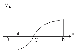
Theorem 2. If the function f(x) is continuous on the interval [ a,b] and at the ends of the segment takes values ​​of different signs, then there is such an internal point x 0 segment [ a, b], in which the function turns to 0, i.e. $ x 0 Î ( a, b) (f(x 0) = 0).

This theorem states that the graph of a function y = f(x), continuous on the interval [ a, b], intersects the axis Ox at least once if the values f(a) And f(b) have opposite signs. So, (Fig. 1.16) f(a) > 0, f(b) < 0 и функция f(x) becomes 0 at points x 1 , x 2 , x 3 .

Theorem 3. Let the function f(x) is continuous on the interval [ a, b], f(a) = A, f(b) = B And A¹ B. (Fig. 1.17). Then for any number C, enclosed between the numbers A And B, there is such an interior point x 0 segment [ a, b], What f(x 0) = C.

Consequence. If the function f(x) is continuous on the interval [ a, b], m– smallest value f(x), M– the greatest value of the function f(x) on the segment [ a, b], then the function takes (at least once) any value m, concluded between m And M, and therefore the segment [ m, M] is the set of all function values f(x) on the segment [ a, b].

Note that if a function is continuous on the interval ( a, b) or has on the segment [ a, b] discontinuity points, then Theorems 1, 2, 3 for such a function cease to be true.

In conclusion, consider the theorem on the existence of an inverse function.

Theorem 4. Let f(x) is continuous on the interval X, increases (or decreases) by X and has a range of values Y. Then for the function y = f(x) there is an inverse function x= j(y), defined on the interval Y, continuous and increasing (or decreasing) by Y with multiple meanings X.

Comment. Let the function x= j(y) is the inverse of the function f(x). Since the argument is usually denoted by x, and the function through y, then we write the inverse function in the form y =j(x).

Example 1. Function y = x 2 (Fig. 1.8, a) on the set X= }